I had the honor of presenting to a full house at FOSS4G-NA 2013 this May. This is a rough transcript of that presentation. Just like my talk at the Big Data Deep Dive, no recording was made, as far as I’m aware. So just like that transcript, this is a recitation from memory.

The deck is available on slideshare, and embedded at the bottom of the post.

I want to speak this morning about a nights-and-weekends project I’ve been cooking since February. While I work on the HBase team at Hortonworks, this project is only tangentially related to what I do. The project is called Tilebrute, it’s a tool for generating map tiles using Apache Hadoop. In part, I wanted to learn some python and the GIS libraries available in that language. More so, I hope it will act as a learning tool and launching point for some of you who don’t have experience with Big Data technologies and are looking for help getting started. I hope it can also solve the last mile problem from someone who wants to take their Hadoop application from their laptop or local cluster into the cloud.

This whole thing started last year at this same conference. I was entirely new to GIS and came hoping for an introduction to the space. One of the talks I attended was titled ”Rendering the World,” presented by Young Hahn from Mapbox. He talked about the computational challenge of rendering, storing, and serving maptiles; this being a service offered by their business. As they say, “when you have a hammer, everything looks like your thumb.” I came away from that talk thinking “this is totally a Hadoop-able problem,” but not with a concrete project for experimentation.

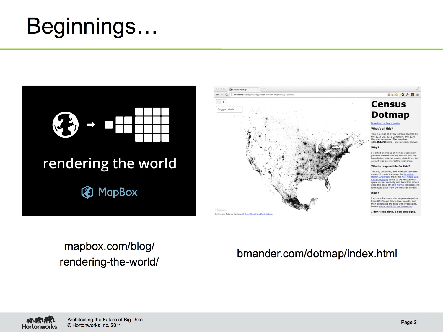
Fast-forward to January of this year. Via the Twitters, a project called the ”Census Dotmap” by Brandon Martin-Anderson came to my attention. “Ah hah!” I thought, “this is perfect!” Mr. Martin-Anderson was considerate enough to write up some details about his process and even provided code samples in the form of some github gists. What really caught my attention was the difficulty of sorting his intermediary data and the overall time it took to render his tileset. If nothing else, Hadoop is a distributed sorting machine and I was certain I’d be able to use it to distribute the application effectively.

Before I go further, let me start by defining some terms. As I mentioned earlier, I have no background in GIS, so I want to make sure you understand my meaning for some of these terms. In particular, Cartography, for the context of this project, means rendering map tiles from some kind of geographic data. In this case, that geographic data will be map coordinates sampled from the source data. Likewise, Cloud, for the purpose of this project, has nothing to do with condensed water vapor. Instead, I’m talking about consuming computational and data storage resources on demand. For this project, I used AWS as the cloud vendor because they’re the provider with whom I’m most familiar. Tilebrute uses Hadoop as the glue for presenting the cartography application in a cloud-consumable format. More on that in a minute. First a little background.

People talk about Apache Hadoop as a single tool, but it’s actually composed of two fundamental parts. The Hadoop Distributed Filesystem (HDFS), provides distributed, redundant storage. HDFS uses the filesystem analogy rather than the table analogy used by databases. It presents a directory structure with files, user permissions, &c. It’s optimized for high throughput of large data files – in a filesystem, files are composed of storage blocks on disk. In the usual desktop filesystems like ext3, the block size is on the order of 4k. HDFS has a default blocksize of 64mb.

The other Hadoop component is Hadoop MapReduce. MapReduce is the computational framework that builds on HDFS. It provides a harness for writing applications that run across a cluster of machines and a runtime for managing the execution of those applications. Its operation is batch-oriented – it sacrifices latency for throughput and is designed to compliment the features of HDFS. MapReduce applications are generally line- or record-oriented. Both HDFS and MapReduce are open source implementations of the data storage and computation systems described by papers published by Google almost 10 years ago.

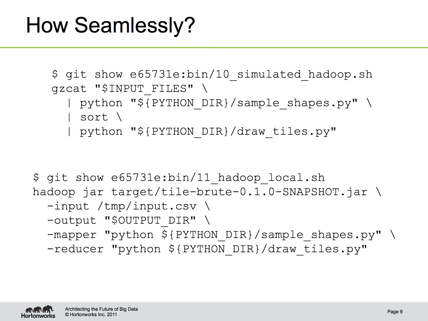
Data running through a MapReduce application is described in terms of key-value pairs. This diagram is the best depiction of the MapReduce framework I’ve found. All we really care about for the purposes of Tilebrute are the map step, the sort, and the reduce step. Thus, MapReduce can be boiled down to a simple analogy to UNIX pipes. Input is piped into the mapper application. Its output is sorted and before being passed into the reducer. Hadoop then handles collecting the output. Normal Hadoop applications are written in Java, but Hadoop also provides an interface for executing arbitrary programs, called Streaming. With Hadoop Streaming, if you can write a program that reads from standard in and writes to standard out, you can use it with Hadoop. The UNIX pipes analogy translates quite seamlessly into a Hadoop Streaming invocation.

Enough about Hadoop, let’s get to the code! Again, the whole project is open source and available on github.

The Brute is built on Hadoop Streaming with Python. It uses a couple well-known Python GIS libraries. GDAL is used to pre-process the input before it’s fed to Hadoop, Shapely for some simple geometry functions, and Mapnik to render the final tiles. There is a touch of Java in Tilebrute: there’s a Hadoop output extension that can emit tiles in the correct z/x/y.png tile path. For cloud configuration and deployment, it uses a project called MrJob, open sourced from Yelp. It has a ton of features for writing Hadoop applications in Python, of which Tilebrute uses almost none of them – it’s a Streaming application in the simplest form. There’s also a touch of Bash, mostly so that I could remember what commands I ran last weekend.

The input to Tilebrute are the TIGER/Line shapefiles provided by the US Census Bureau. Well, almost. Hadoop is line-oriented, remember, and shapefiles are optimized for a different access pattern. I used ogr2ogr to transform the input into simple CSV records, preserving the feature geometry. The only fields we care about in the output are the first – the geometry – and the last – the population count for that feature.

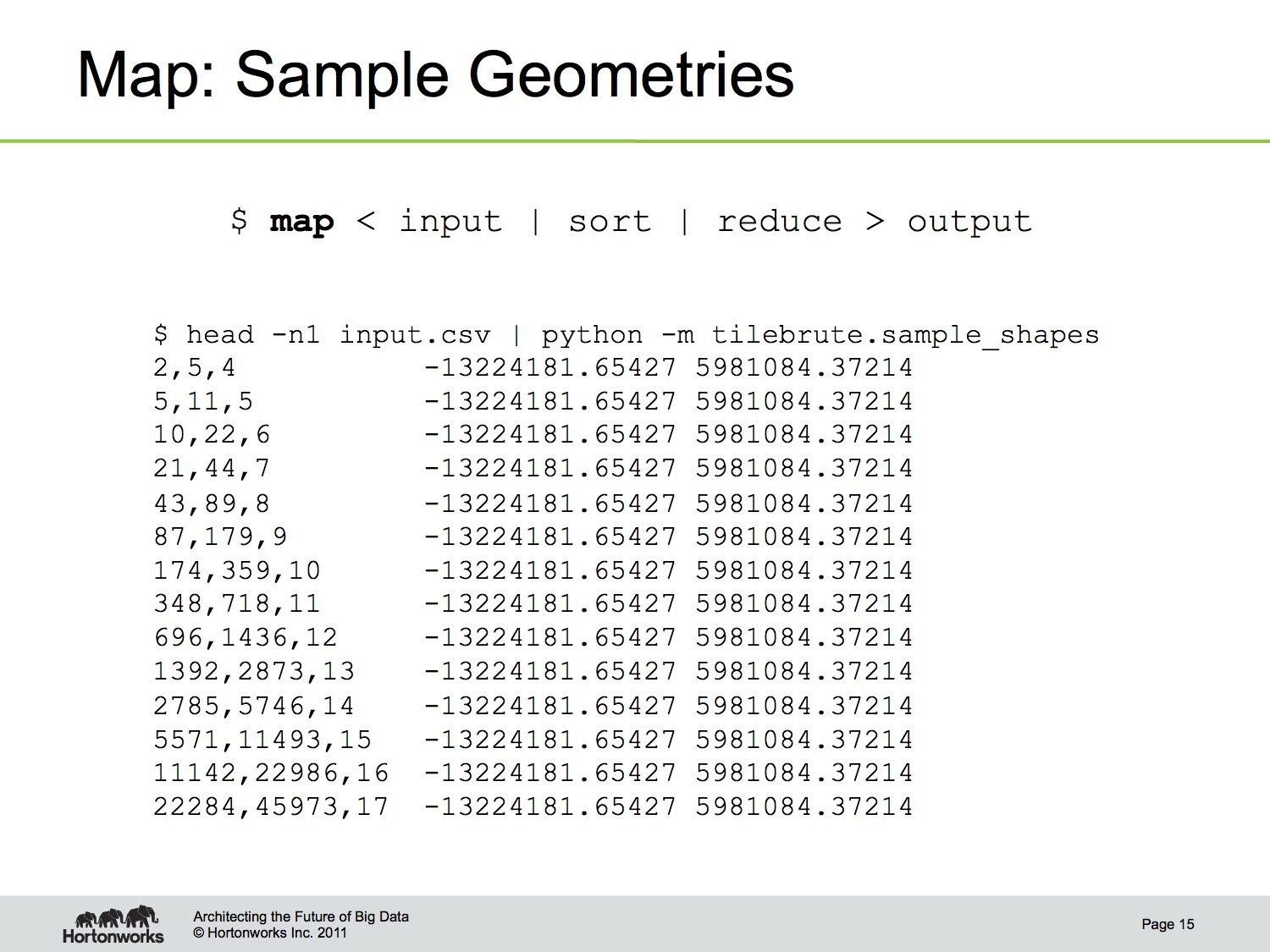
Remember, everything in Hadoop is described in terms of key-value pairs. For the map step, we read in each feature record and sample the points from that geometry. If the population field is 10, the mapper generates 10 random points within the geometry. Those points are associated with a tileId. In this case, that means the tile’s zoom, x, and y coordinates in the tile grid. I considered using quadkeys for the tileId, but the total ordering isn’t necessary for our purposes. Here’s an example of the mapper output. In this case, zoom levels 4-17 are being generated and the same point is emitted once for each zoom level.

The sort step is provided for us by Hadoop. Specifically, it means that all the points for a single tile are made available at the same time for the reducer to consume. This a fundamental semantic of the MapReduce framework.

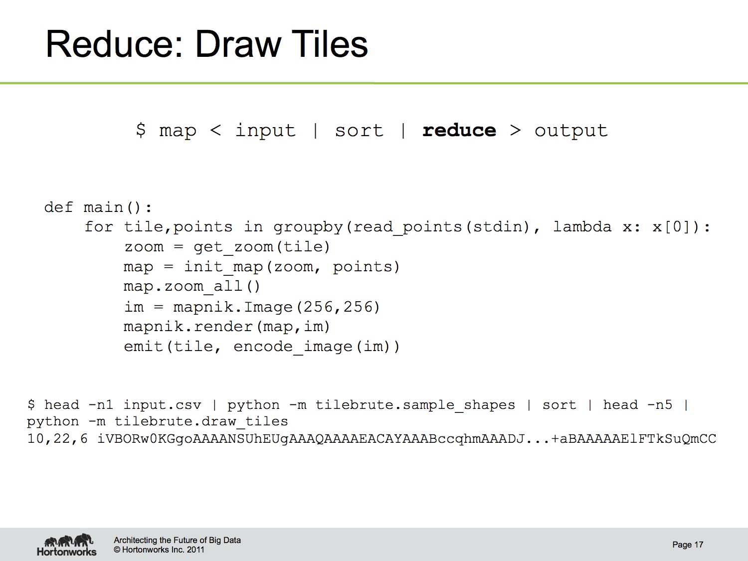
The reducer takes that list of points for a single tile and feeds them into mapnik to render the tile. This is where the most application-level optimization work has gone into this project. In particular, making sure mapnik is able to consume 25 or 30 million points without choking is critical for this to work. Special thanks to Dane Springmeyer for his mapnik help! The reducer output is the tileId and the png tile. Hadoop Streaming, the way I’m using it so far, is line-oriented and textual, so the png binary is base64-encoded.

This snippet is the only Java code in the whole project. It’s the Hadoop output plugin for consuming the tileId and encoded png and turning them into a tile file on the output filesystem.

To the cloud! (I always wanted to say that in a presentation)

AWS provides two basic services: EC2 and S3. EC2 is the on-demand computation service. It provides virtual machines, allocated (and billed) according to hardware profiles. These profiles are called “instance types.” In this case, I’ve used the two instance types m1.large and c1.xlarge. I’ve stuck to these two types because they’re both 64-bit architectures; working with only a single architecture simplified my deployment automation scripts.

S3 is the storage service that compliments EC2. It’s a distributed, redundant key-value store. Of particular interest, Hadoop supports S3 as a filesystem, so it can be used pragmatically as a drop-in replacement for HDFS. The S3 service also provides HTTP hosting, which will make it easy to host the map tiles in web applications once they’re generated.

The last service employed by the Brute is EMR. It’s an add-on service, built on top of EC2 and S3. It handles installation of Hadoop on the EC2 nodes for us, and also standardizes the provisioning of clusters, running of jobs, &c. The biggest downside is that it runs an older version of Debian that doesn’t have the latest version of our tools available. We work around this by building and deploying the software ourselves, all automated with simple scripts run as “bootstrap actions” at cluster launch time. This automation is also standardized by EMR’s API.

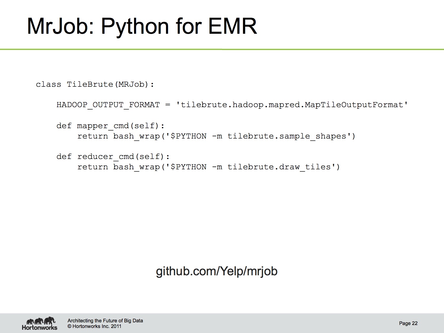
The last component is the MrJob entry point. This is where the Streaming application is defined. As you can see, it’s a short Python file that specifies the mapper, reducer, and our custom output format. It also has a configuration file which holds all the cluster launch details for us. I’ve included a couple different cluster configurations, along with some comments reasoning through the settings.

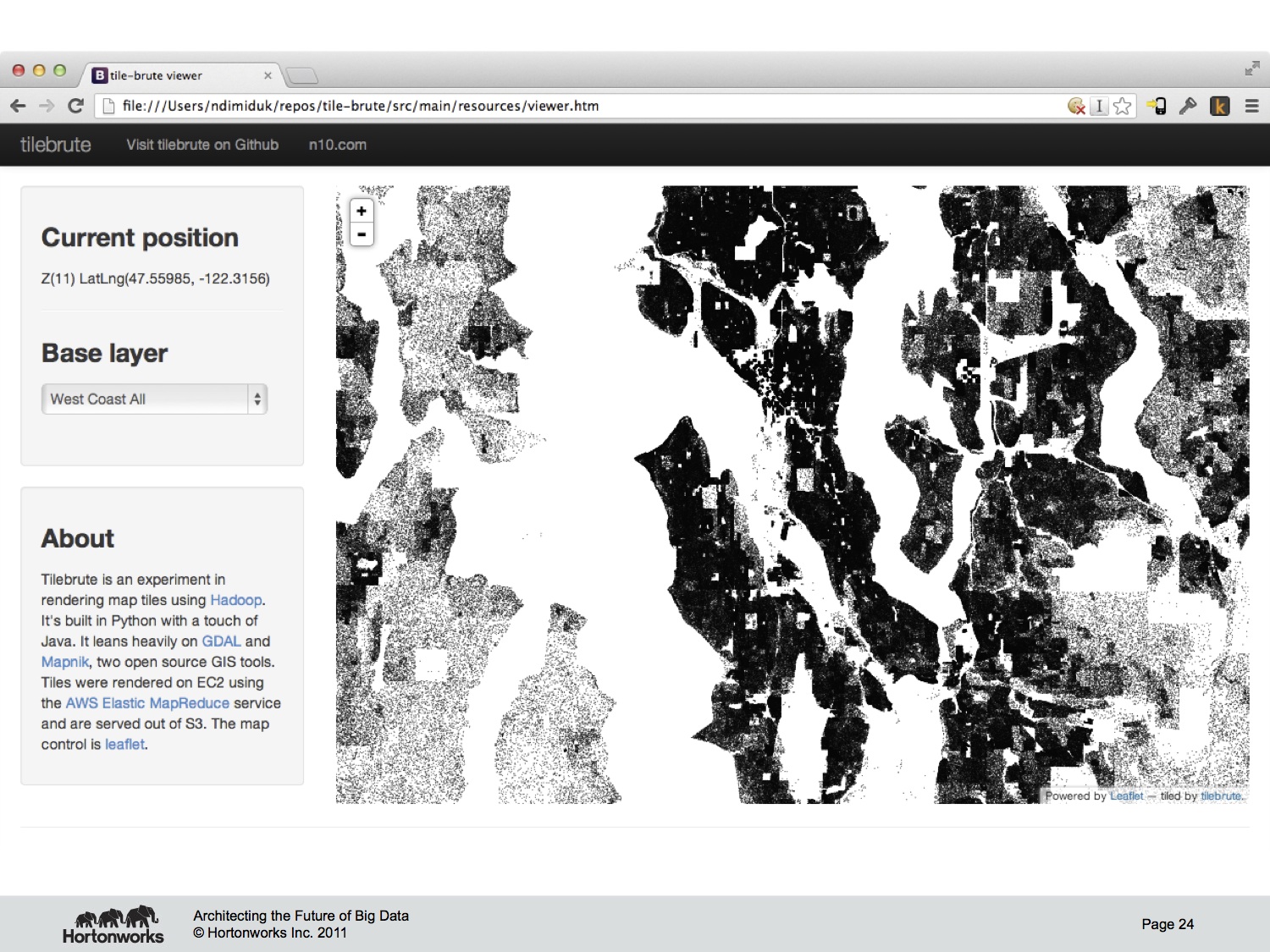
On to the results. Being prepared for total conference wifi fail, this is a screenshot of the Tilebrute output. I hacked up a simple tile viewer using Leaflet, and host it out of S3 right beside the Hadoop output tiles. Here’s the same tile, one from Google Maps and the others from bmander and the Brute. As you can see, the same input data sampled to roughly the same output – it’s hard to tell that they are indeed different.

The whole project comes together in less than 250 lines of code, and only 150 lines if you omit all the shell glue. In this way, Tilebrute succeeds in its goal of being a simple project for demonstrating use of Hadoop Streaming for cartographic applications.

Don’t stare too hard at these performance numbers. I kicked off these jobs while listening to the lightning talks last night and haven’t had a chance to evaluate them properly or make a pretty graph. The point I’m trying to show is that Hadoop lets you scale the exact same application up from running on a single machine with a small input set to multiple machines crunching a much larger dataset. This is the kind of flexibility in scale that Hadoop is designed to provide, and why Hadoop is often used as an example “cloud application.”

As for improvements, I’ve started a todo list. The big thing with Hadoop applications is that you have two levels of optimization. At the cluster level, there’s “macro” tuning of cluster configurations. Considerations here are things like how many concurrent processes to run and balancing those processes between map and reduce tasks. There’s also the matter of reducer “waves,” taking into consideration the amount of data skew as it spreads across the reducers. The idea is to have all reducers finish at about the same time so as to minimize wasted compute time. There’s also application-level, “micro” tuning. This is your standard tight-loop optimization and other such considerations. Smarter input sampling and mapnik library improvements both fall into this category. Other open ideas include writing to S3 more efficiently and possibly using MBTiles format instead of writing raw map tiles.

That’s Tilebrute, thanks for listening! Any Questions?